Linear regression with julia

This post is a tutorial on how to do linear regression with single and multiple variables using Julia in the best possible way. I have divided the tutorial in small steps and code snippets with explanations where ever possible. I have used my Jupyter notebook for this post.

using DataFrames, CSV
using Plots
pyplot();

Lets get our Data!

This is a sample data stored in a CSV file ex1data1.txt

You can get the data here.

## This is how we read data from a CSV file
## The first column is the population of a city and the second column is the profit of a food truck in that city.
## A negative value for profit indicates a loss.
data = CSV.read("ex1data1.txt");

## Renaming columns of the dataset
## This is how we can rename columns of a DataFrame in Julia v1.0
newnames = ["Population", "Profit"];
names!(data, Symbol.(newnames));

## If you want to see a small part of the data so as to know how it looks like
head(data)

	Population	Profit
1	5.5277	9.1302
2	8.5186	13.662
3	7.0032	11.854
4	5.8598	6.8233
5	8.3829	11.886
6	7.4764	4.3483

## Splitting the features i.e. population in 10,000s here (X) and the function values i.e. profit in $10,000s here (Y)
X = data[:Population];  #features
y = data[:Profit];  #Y-values

## To see number of training samples
num_tr_ex = length(y); #96

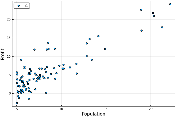
It is helpful if you can plot and visualize the data

# Simple Scatter plot using PyPlot
scatter(X,y, xaxis="Population", yaxis="Profit")

Linear Regression with single variable ( profit = f (Population) )

using GLM
linearRegressor = lm(@formula(Profit ~ Population), data)

StatsModels.DataFrameRegressionModel{LinearModel{LmResp{Array{Float64,1}},DensePredChol{Float64,LinearAlgebra.Cholesky{Float64,Array{Float64,2}}}},Array{Float64,2}}

Formula: Profit ~ 1 + Population

Coefficients:
             Estimate Std.Error  t value Pr(>|t|)
(Intercept)   -4.2115  0.635259 -6.62958    <1e-8
Population    1.21355 0.0702113  17.2842   <1e-30

Here we are using GLM (Generalized Linear Models) Julia package which is based on the GLM package for R. predict() predicts the values of the dependent variable according to the fitted model (like Profit in our case) lm() is an alias function to fit a linear model for the given data.

linearFit = predict(linearRegressor)
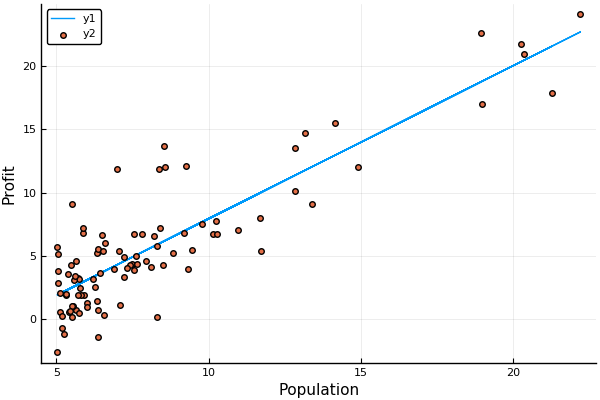
## To see how the model is fitted with the data
plot(X,linearFit)
scatter!(X,y, xaxis="Population", yaxis="Profit")

To predict the profit where the population is say 35,000 and 70,000. We can use the coefficients from the above model

newX = DataFrame(Population = [3.5, 7])
predict(linearRegressor, newX)*10000

2-element Array{Float64,1}:
   359.11383255145427
 42833.2677193441    

Linear Regression with multiple variables

Here the data is house price based on size and number of bedrooms.

You can get the data here.

## This is how we read data from a CSV file
## The file ex1data2.txt contains a training set of housing prices in Port- land, Oregon.
## The first column is the size of the house (in square feet),
## the second column is the number of bedrooms, and the third column is the price of the house.
data_mul_var = CSV.read("ex1data2.txt");

## Renaming columns of the dataset
## This is how we can rename columns of a DataFrame in Julia v1.0
new_names = ["Size","Bedrooms","Price"];
names!(data_mul_var, Symbol.(new_names));

## How the data looks ?
head(data_mul_var)

	Size	Bedrooms	Price
1	1600	3	329900
2	2400	3	369000
3	1416	2	232000
4	3000	4	539900
5	1985	4	299900
6	1534	3	314900

# Seperating Features and labels
X_ = data_mul_var[:,[:Size,:Bedrooms]];
y_ = data_mul_var[:Price];
num_tr_ex = length(y_);

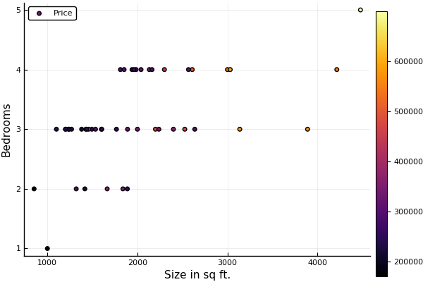
# Plotting Data for Visualization
@df data_mul_var scatter(:Size,:Bedrooms, zcolor= :Price, xaxis = "Size in sq ft.", yaxis="Bedrooms", lab="Price")

Feature Scaling is necessary in this case if we are using gradient descent and want the model to converge more quickly because the features (bedrooms and size are in different scale).

If we are using GLMs linear model then it takes care of the scaling implicitly.

normal_value = (value - mean)/(max - min)

Note: To fit in the linear function y = mx + b, we need to add b (bias in the features) Here the GLM linear model takes care of the bias as we can see the Formula in the following model output is Price ~ 1 + Bedrooms + Size. Here 1 is the added bias.

## Fitting the Linear Model to the data
linearRegressor_mul = lm(@formula(Price ~ Bedrooms + Size), data_mul_var)

StatsModels.DataFrameRegressionModel{LinearModel{LmResp{Array{Float64,1}},DensePredChol{Float64,LinearAlgebra.Cholesky{Float64,Array{Float64,2}}}},Array{Float64,2}}

Formula: Price ~ 1 + Bedrooms + Size

Coefficients:
             Estimate Std.Error   t value Pr(>|t|)
(Intercept)   87807.8   42121.6   2.08463   0.0431
Bedrooms     -8186.38   15571.9 -0.525714   0.6018
Size          138.756   14.9057    9.3089   <1e-11

To predict the price where the no. of bedrooms is say 3 and size is 1650 sq ft. We can use the coefficients from the above model

newX = DataFrame(Bedrooms = [3], Size = [1650])
predict(linearRegressor_mul, newX)

1-element Array{Union{Missing, Float64},1}:
 292195.8009513173

Normal Equation method for linear regression

coeff = inv(X’ * X) * X’ * y

## Converting the Data Frame to Arrays for matrix multiplication
## Adding a column of 1s for the Bias
x = convert(Array, data_mul_var[:,1:2]);
z = ones(length(y),1)
x = hcat(z,x)
y = convert(Array, data_mul_var[:Price]);

## Normal equation method to find out the optimum coefficients for which the cost is zero
## (No need for feature scaling here) But we need to add a Bias ( a column of 1s)
coeff = inv(x'*x)*x'*y

3-element Array{Any,1}:
 87807.7501932388    
   138.75587841570885
 -8186.382875946652  

Predicting the price with the coefficients obtained

reshape([1,1650,3],(1,3))*coeff

1-element Array{Any,1}:
 292195.8009513184

The price is almost same as what we calculated with the linear regression model.

Thank you! Thats all for the post. Stay tuned for more. :D